
Formula Time Series
The TSM supports formula based time series. All Microsoft .Net Framework functions are supported in VB.Net notation. Additionally, user-defined functions can be created and used in VB.Net.
Editing and calling a formula is carried out in the Edit tab for time series. It can be reached via Search -> Edit.
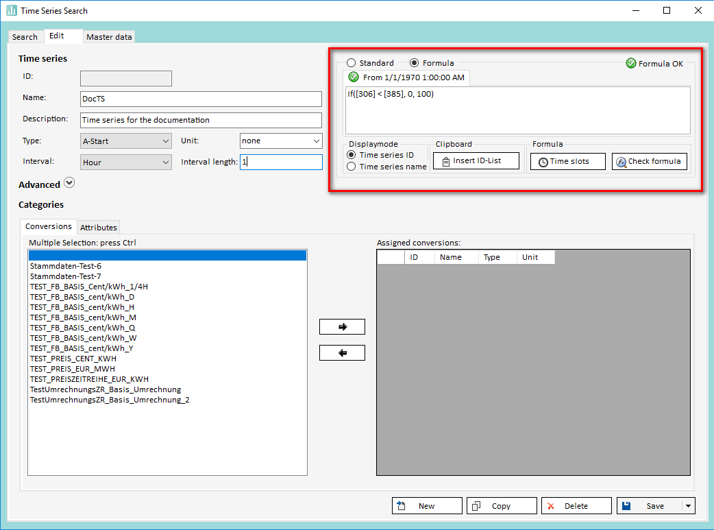
When the cursor is located in the Formula text field, you can have a list of all available functions by pressing the space bar.
Overview formula time series
Formula time series are defined by the underlying formula. This formula contains the calculation rule. The time series definition of a calculated time series is saved in the data base like all other time series. Additionally, the definition includes a formula. If the time series definition is changed, an archive entry with corresponding time mark is created in the data base to secure auditing acceptability. Thus, also historical outcomes can be accessed and displayed. When time series are read-out, they are calculated according to the formula and the outcome is provided.
Calculation rules based on other time series can be displayed with formulas. Time series or numbers can be calculated using basic arithmetical operations and functions (+, -, *, /). Moreover, customer specified functions can be implemented.
Syntax of formulas
Formulas are administered in simple text. When a time series is read-out, the formula is compiled and calculated by the HAKOM Framework. The syntax is identical to the one used in VB.Net. Moreover, all functions from Math Namespace can be used:
(https://docs.microsoft.com/en-us/dotnet/api/system.math?redirectedfrom=MSDN&view=netframework-4.7.2).
Operators
Formulas support the following operators:
| + | - | * | / | ^ | Mod |
Additionally the following relational operators are supported:
| = | <> | < | > | <= | >= |
e.g.: 3 + 5 * 2 results in a time series that has the constant value of 13
Brackets are supported as well:
e.g.: (3 + 5) * 2 results in a time series that has the constant value of 16
Including other time series
Time series can be included in a formula according to the following pattern:
[Time series (name or ID), offset (optional), unit (optional), aggregation (optional)]
| Parameter | Description |
|---|---|
| Time Series | Name or ID of the time series to be referenced. |
| Offset | Extension of the period for which data is loaded in both directions. If an offset n is specified, the data n interval steps before the time series start and n increments after the time series end are also loaded. This additionally loaded data is then available for calculations. |
| Unit | Unit into which the data of the referenced time series should be converted. |
| Aggregation | Aggregation rule to be used when aggregating the data of the referenced time series (applicable if calculation interval is different from the interval of the time series). |
When using time series in formulas using square brackets, a data element is passed. In addition to the values ([8765].Value) of the time series, this contains the status ([8765].Flag) of the values, the from and to date ([8765].fromDate and [8765].toDate) and the index of the time series ([8765].Index).
For all operators mentioned above under "Operators" the following rules apply:
- Comparison/calculation of a referenced time series with another time series also returns a data element as a result.
- Comparison/calculation of a referenced time series with an integer-value returns a data element as the result.
- Comparison/calculation of a referenced time series with a double-value returns a data element as the result.
- Calculation may be performed using the value of a time series directly instead of the data elements (By using [time-series-id].Value instead of just [time-series-id]), This returns a double-value as the result.
Examples
Example 1
Only the ID of a time series is used here:
[4711]
When it is loaded, the formula time series returns the same data as the time series 4711.
Example 2
Here the ID of a time series and an offset are passed in order to use the "Lead" function:
Lead([4711, 2], 2)
The formula time series assumes the data of the time series 4711 when loading. Additionally the data 2 interval steps before the "from" date and 2 interval steps after "to" date. The "Lead" function shifts the data by two interval steps, which is made possible by the additionally loaded data outside the "from" and "to" data.
Example 3
Here the ID of a time series, an offset and a unit are passed:
[4711, 0, kW]
When the formula time series is loaded, it returns the values of time series 4711 converted to kW.
Example 4
Here the ID of a time series, an offset, a unit and an aggregation are passed:
[4711, 0, "", Sum]
When the formula time series is loaded, it returns the values of time series 4711. If data is aggregated (e.g. because the intervals of the time series are different), the sum of the data is calculated.
Example 5
Here the values of several time series are used in combination with some of the supported operators:
[4711]*3+[123]+0.22
Here, the formula time series assumes the value of time series 4711 multiplied by three and summed with the value of time series 123 and the value 0.22.
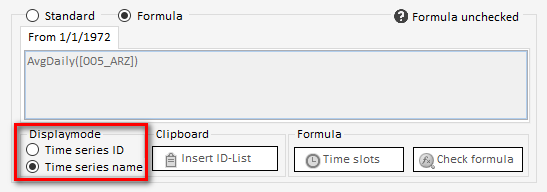
If the name of a time series is entered into the formula editor, it will be automatically changed to that time series ID. This guarantees that no unwanted side effects occur should this time series be renamed. By choosing the displaymode "Time series name" it is possible to display the name rather than the ID. In this mode it is not possible to make changes to the formula.
Specification of Formula Time Series
Interval
Formula time series are calculated based on their specified interval. All time series referenced in the formula will be loaded in this given interval before a
Example: Evaluating load profiles with the load stored in hourly intervals and price time series stored in half hourly interval.
Scenario 1 – Formula time series with interval: Hour
Calculation: Load profile (hourly resolution) * price time series (averaged to hourly resolution)
Result: A formula time series in hourly resolution
Scenario 2 – Formula time series with interval: Day
Calculation: Load profile (averaged to daily resolution) * price time series (averaged to daily resolution)
Result: Formula time series in daily resolution
-> This consequences in a wrong result, as only daily average values are calculated.
Scenario 3 – Formula time series with interval: Hour, Read-Out with interval: Day
Calculation: Load profile (averaged to hourly resolution) * price time series (averaged to hourly resolution)
Intermediate result: Formula time series in hourly resolution
Result: Formula time series read-out in daily resolution
-> This leads to a correct result, as the daily value of the formula time series consists of accumulated hourly values.
Units
It is possible to state a unit in the formula of a time series.
e.g. [530379,-3,KW,Average] converts the data of the time series 530379 from MW to KW, defers the time series for -3 intervals and calculates the average which is generated across the resolution of the formula time series with the values of the times series 530379.
Please note that the conversion of units has to be plausible (Conversion from MW to Euro or percentage is not possible.).
Functions in EvalComponent
There are several .VB files in the BIN directory of the TSM which names start with EvalComponent. The functions which can be called in the formula editor are located in these files. They are deposited in .Net syntax.
Formulas that are public functions in an EvalComponent, will be displayed in the TSM's formula editor through the Intellisense. By pressing the space bar the Intellisense will show you a list of all public functions.
Example function in EvalComponents:
Public Function If(ByVal a As Boolean, ByVal b As Double, ByVal c As Double) As Double
   If a Then Return b Else Return c
End Function
Calling the formula in the TSM:
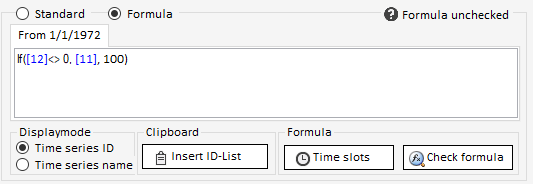
In this case, when calling the formula, the operators <> trigger a comparison of the values from the time series [12] are unequal 0.
The outcome is a Boolean value (True / False). By means of this Boolean, the function decides if when True the value from time series [11] is delivered, or when False the value “100”.
Standard functions
The TSM bin-folder contains files whose names start with "EvalComponentHAKOM". These files contain the standard functions delivered by Hakom.
| Name | Parameter | Example | Description |
|---|---|---|---|
Average | Average(ByVal ParamArray data As Data())* | Average([15],[16]) | Returns the average of the passed values. In the example, this would be the average of the two time series |
AverageLeadLag | AverageLeadLag(ByVal data As Data, ByVal Shift As Int32())* | AverageLeadLag([16748],6) | Returns the average values shifted by the amount of interval steps (shift) given. |
AvgDaily | AvgDaily(ByVal data As Data)* | AvgDaily([15]) | Returns the average value of a day. |
AvgOfRange | AvgOfRange(ByVal data As Data, ByVal shiftFrom As Integer, ByVal shiftTo As Integer)* | AvgOfRange([195829],6,12) | Returns the average value of the given time series between shiftFrom and shiftTo. |
BestValue | BestValue(ByVal ParamArray dataArray As Data())* | BestValue([15],[16]) | This function returns the "best" value measured by the flag of that value. If one time series has a value with the flag "missing" and the others value has "valid" for the same period, the valid one will be returned. If both have the same flag then the one of the first parameter is returned. |
ConstantMaturity | ConstantMaturity(ByVal data As Data, ByVal maturity As Integer, ByVal maturityInterval As Components2016.TimeSeries.TimeSeriesInterval, Optional ByVal exact As Boolean = True) ConstantMaturity(ByVal data As Data, ByVal maturity As Integer, Optional ByVal exact As Boolean = True) | ConstantMaturity([4231],4) ConstantMaturity([4231],4,Components2016.TimeSeries.TimeSeriesInterval.Hour) | This function is used to combine the different quotations of a quotation time series. You can find an example of how it works below this table. |
FromNow | FromNow(ByVal value As Double) | FromNow(100) | Returns the passed value as long as the interval it is returned to lies in the future. Otherwise 0 is returned. On 01.01.2019 at 06:00 the formula time series has the value 0 for all entries until 01.01.2019. From the next interval on it has the value 100. |
GetMyAttributeValue | GetMyAttributeValue(Attribute name, [Date/Time]) | GetMyAttributeValue("Test_Attribut_1") | Returns the value of an attribute assigned to the formula time series. If multiple time slices are stored, you may pass an additional parameter to specify for which time the value should be retrieved. If no value is given, it uses the current date/time. |
| GetAttributeValue | GetAttributeValue(Time series ID, Attribute name, [Date/Time]) | GetAttributeValue(101752,"Test_Attribut_1", new DateTime(2019,01,01,23,0,54) | Returns the value of an attribute assigned to the formula time series. If multiple time slices are stored, you may pass an additional parameter to specify for which time the value should be retrieved. If no value is given, it uses the current date/time. |
GD „Gleitender Durchschnitt“ (=Moving Average) | GD(ByVal data As Data, ByVal average As Integer, ByVal offset As Integer)* GD(ByVal data As Data, ByVal average As Integer, ByVal offset As Integer, ByVal valid As Integer)* | GD([195829], 7, 0) GD([195829],2,0,3) | GD with 3 parameters (without "valid"): This function calculates the moving average over the given amount of raster steps ("average") using the given offset ("offset") in interval steps. The interval used in the calculation is the one used as resolution of the template. E.g.: GD([195829], 7, 0): given a resolution of one day, the moving average of the time series over 7 days without offset is returned. The 8th day will have the average of days 1-7. The 9th day the average from 2-8 and so on. GD with 4 parameters (with "valid"): The additional parameter sets the amount of periods that will acquire the calculated value. Attention: The interval used in the calculation is always month! E.g.: GD([195829],2,0,3): The moving average of 2 month without offset is calculated and the resulting value is acquired for the next 3 months. |
Lag | Lag(ByVal data As Data, ByVal Shift As Integer)* | Lag([15],48) | The time series values are shifted ahead by the amount of interval steps (Shift) given in the formula. |
LagDaily | LagDaily(ByVal data As Data, ByVal Shift As Integer)* | LagDaily([15],2) | The time series values are shifted ahead by the amount of days (Shift) given in the formula. |
Lead | Lead(ByVal data As Data, ByVal Shift As Integer) | Lead([15],-1) | The time series values are shifted backwards by the amount of interval steps (Shift) given in the formula. |
LeadDaily | LeadDaily(ByVal data As Data, ByVal Shift As Integer)* | LeadDaily([15],2) | The time series values are shifted backwards by the amount of days (Shift) given in the formula. |
MaxDaily | MaxDaily(ByVal data As Data) | MaxDaily([17]) | Calculates the maximum value on a daily basis. |
MaxOfRange | (ByVal data As Data, ByVal shiftFrom As Integer, ByVal shiftTo As Integer)* | MaxOfRange([195830],6,12) | Returns the maximum value of a time series within the parameters shiftFrom to shiftTo. |
MinDaily | MinDaily(ByVal data As Data)* | MinDaily([17]) | Calculates the minimum value on a daily basis. |
MinOfRange | MinOfRange(ByVal data As Data, ByVal shiftFrom As Integer, ByVal shiftTo As Integer)* | MinOfRange([195830],6,12) | Returns the minimum value of a time series within the parameters shiftFrom to shiftTo. |
OffPeak | OffPeak(ByVal data As Data) | OffPeak([195830]) | Returns the values of Off-Peak values (Mo-Fr, 08:00 pm - 08:00 am, Sa and Su) of the given time series. Returns 0 missing for all other times. |
Peak | Peak(ByVal data As Data) | Peak([200]) | Returns the values of Off-Peak values (Mo-Fr, 08:00 am - 08:00 pm) of the given time series. Returns 0 missing for all other times. |
| Sum | Sum(ByVal data As Data) | Sum([1447]) | Returns the sum of values that are saved on the referenced time series. |
TSA | TSA(Attributes As String, Unit As String) | TSA("DocCategory","kW") | Returns the aggregate of the given attribute (It has to be of type "Category!) converted to the given unit. The values per interval will always have the "worst " Flag that one of the time series that was assigned this attribute has. E.g.: If the flag of a time series from 01:00-02:00 is "valid" and that of another one is "missing", the formula time series will have the flag "missing" for this period. |
TSAA | TSAA(Unit As String, bestStatus As Boolean, ParamArray Attributes() As String) | TSAA("kW",true,"DocAttribute") | The TSAA formula works similar to the TSA formula, but can have any type of attribute as parameter. Additionally a boolean can be passed. It states, if the flag for a period should be "valid", if at least one of the time series used in the aggregation has a flag other than "missing" or "faulty" for this period. It is possible to pass multiple attributes seperated by comma. Only time series that are assinged all given attributes will be used for the aggregation. |
TSCA | TSCA(Unit As String, ParamArray Attributes() As String) TSCA(Unit As String, bestStatus As Boolean, ParamArray Attributes() As String) TSCA(TimeSeriesName As String, Unit As String, bestStatus As Boolean, ParamArray Attributes() As String) | TSCA("kW","DocCategory") TSAA("kW",true, "DocCategory","DocCategory_2") TSCA("Doku ZR%","kW",true, "DocCategory","DocCategory_2") | The TSCA formula works similar to the TSA formula. Additionally a boolean can be passed. It states, if the flag for a period should be "valid", if at least one of the time series used in the aggregation has a flag other than "missing" or "faulty" for this period. It is possible to pass multiple attributes seperated by comma. Only time series that are assinged all given attributes will be used for the aggregation. It is also possible to pass the name of a time series (also incl. wildcard) as parameter. |
UntilNow | UntilNow(ByVal value As Double) | UntilNow(100) | Returns the passed value as long as the interval it is returned to lies in the past. Otherwise 0 is returned. On 01.01.2019 at 06:00 the formula time series has the value 100 for all entries until 01.01.2019. From the next interval on it has the value 0. |
ValidAvg | ValidAvg(ByVal data As Data)* | ValidAvg([2342]) | Aggregates the averaged time series values into the predefined resolution (Hour). Only values whose flag is not "missing" are taken into account. |
ValidAvgLeadLag | ValidAvgLeadLag(ByVal data As Data, ByVal Shift As Int32)* | ValidAvgLeadLag([2342],6) | This function works like ValidAvg extended by a shift. |
ValidIntegral | ValidIntegral(ByVal data As Data)* | ValidIntegral([195829]) | Aggregates the time series values into the predefined resolution (Hour). Only values whose flag is not "missing" are taken into account. |
ValidMax | ValidMax(ByVal data As Data)* | ValidMax([195829]) | Aggregates the time series values into the predefined resolution (Hour) and acquires the maximum value that does not have the flag "missing". |
ValidMin | ValidMin(ByVal data As Data)* | ValidMin([195829]) | Aggregates the time series values into the predefined resolution (Hour) and acquires the minimum value that does not have the flag "missing". |
XChange | XChange(ByVal Name As String, ByVal Unit As String) | XChange("Doku ZR_3","kWh") | Converts the given time series data to the given unit. |
*These functions can be used with an integer instead of a data-type parameter (Lag([123].Index instead of Lag([123])).
Examples
For the following examples the following definitions apply:
There are four different versions of "ConstantMaturity_Data": On 15.02.2019 every quarter of an hour between 06:00:00 AM and 09:00:00 AM.
The resolution of both time series is a quarter of an hour.
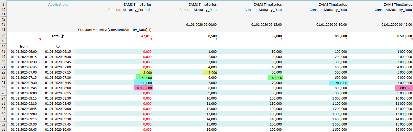
Example 1: The ConstantMaturity Function
ConstantMaturity([ConstantMaturity_Data],0)

How do these values come about?
The function checks, if there is a version of the given time series for the actual period. So for 06:00-06:15 it checks, if there is a version of "ConstantMaturity_Data" of 15.02.2019 at 06:00. Since this is the case, the parameter "maturity" which represents a shift, is applied to this version. In this example maturity is 0 and therefore no shifting happens and the value from 06:00-06:15 is acquired.
The next period is 06:15-06:30. Again the function checks for a version of the given time series at this period and writes it to the formula time series.
From 07:00 there is no more version of "ConstantMaturity_Data" and so the following values are 0 missing.
Example 2: The ConstantMaturity Function With Shifting
ConstantMaturity([ConstantMaturity_Data],4)
The values of the formula time series are calculated as in example 1. Only the parameter "maturity" differs. This means, that the value is still taken from the version at 06:00, which is the actual starting time of the period, but now applying 4 shifts by 15 minutes each, the value from 07:00-07:15 is taken.
After the period from 06:00-06:15 the function continues with the one from 06:15-06:30 and takes the value from the version at 06:15 again applying a shift of 4 periods and so on.
Because there is no version of "ConstantMaturity_Data" before 06:00 the values of the formula time series from 06:00-07:00 are 0 missing.
Example 3: The ConstantMaturity Function With Shifting By Interval
ConstantMaturity([ConstantMaturity_Data],2,Components2016.TimeSeries.TimeSeriesInterval.Hour)
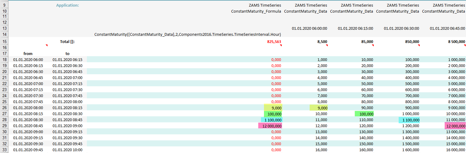
In this example the function was given an additional parameter - an interval (Components2016.TimeSeries.TimeSeriesInterval.Hour). Now maturity has the value 2 and the interval is hour. Again the values are taken from the version that fits the actual periods starting time, but this time they are shifted by two hours.
Individual EvalComponents and Programming
It is possible to create own EvalComponents files. These files should be administered by the user or arranged with HAKOM. Otherwise, it is possible that these special files are not installed when reinstalling. These files can be saved in the folder Custom of the installation package to be picked up for the next installation.
Creation and Syntax
To create an own EvalComponent file, a .vb file has to be created in the Bin directory of the TSM installation. The file name has to start with EvalComponent.
e.g. EvalComponentMyFunctions.vb
Content:
Imports System
Imports HAKOM.Framework.DAL
Imports HAKOM.Framework.Lib
Imports HAKOM.Framework.TimeSeries
Imports System.Collections.Generic
Imports System.Data

Partial Public Class EvalComponent

'own functions

End Class
Attention: Self-made EvalComponents must never be written into the ones delivered by HAKOM (EvalComponentHAKOM.vb, EvalComponentHAKOMOptional.vb, EvalComponentHAKOMReferences.vb)
Value and index functions:
There are two options to apply time series values when calling a function.
Value
The value can be applied directly like in the following example:
Add2(ByVal value Double) As DoubleThe call of this function looks like this: Add2([1234])
In the EvalComponent file the function would look like this:
Private Function Add2(ByVal value As Double) As Double
      Return value + 2
End Function
Index
Moreover, the index of a value can be applied. In this case, not the value is applied but the position of the value in mSourceTSData emanating from the current position. This can be required if an offset shall be used.
Add2(ByVal index As Integer) As DoubleThe call of this function looks like this: Add2([1234].Index)
In the EvalComponent file the function would look like this:
Private Function Add2(ByVal index As Integer) As Double
      Return mSourceTSData(index)(aktLine).Value + 2
End Function
Variables
Variable | Description |
|---|---|
Private aktLine As Int32 | Always accords to the row which currently is calculated. Is used to access contemporaneous values of other time series. Their index and the moment (aktLine) which currently shall be calculated is required in the mSourceTSData array. |
mAktWorstStatus As tsMeterdataStatus | The worst status of all values used for the calculation. If the calculation shall be conducted differently, this variable can be set in an UDF. |
Private mSourceTSData As ITimeSeriesData()() | Contains all time series data (FromDate, ToDate, Value, Flag) of the referred time series in the calculation resolution. |
Private mSourceTSDefDTOs As ITimeSeriesDefinitionDTO() | Contains the definition of the referred time series. |
Private mSourceTSDTOs As ITimeSeriesDTO() | Contains all time series data (Date, Value, Flag) of the referred time series without resolution. It can be used for calculations. |
Private mFormulaTimeSeriesDefinition As ITimeSeriesDefinitionDTO | Contains the definition of the formula time series. |
Private mModTime As UniversalTime | Represents a time, that can be passed when requesting the states (Audit) of time series. |
Private mCalculationTSData() As ITimeSeriesData | Contains all calculated time series data (FromDate, ToDate, Value, Flag) in the calculation resolution. The files in the array are pre-inserted with value 0 and status “Missing” and afterwards successively calculated. |
Private mConnection As IDBConn | Connection to formula time series (can be used for further requests) |
Assembly Cache
The assembly cache can be activated to accelerate the call of functions in EvalComponents.
The functions in the EvalComponent*.vb files are translated into a temporary DLL at every function call. To save the required time for this process, the following entry can be added to HAKOM.Config.
<HAKOMFramework>
    <settings>
		<AssemblyCache>
			%ALLUSERSPROFILE%\HAKOM\TimeSeriesManager\AssemblyCache
		</AssemblyCache>
    </settings>
</HAKOMFramework>
A path where the otherwise temporary DLL would be saved can be defined in the tags <AssemblyCache>. If the EvalComponent data respectively the formula are not changed until the next call of a formula time series, this DLL is reused.