Time Series Types in Comparison

In HAKOM TSM there are different time series depending on the area of application. They can be categorised according to the following criteria:

1. Based on the dimension of data (see chapter: Dimensions of Time Series)

2. Based on the type of time series (see chapter: Types of Time Series)

An additional option is the possibility of compressed data storage. This can be activated with the property "Compression". Detailed information can be found on the following page: Time Series Compression

Furthermore, there are two additional special types of time series, formula time series and conversion time series. Detailed information can be found on the following pages: Formula Time Serie and Units and Aggregation Rules

Dimensions of Time Series

The HAKOM TSM supports following different modes of time series:

• Simple time series without any additional dimension

• Audit time series with historisation of data

• Quotation time series - allows values on a time series with a validity for a given date/time

The mode of a time series can be controlled by setting any of the three properties "Audit" and "Quotation". These settings can also be combined. The following table provides a respective overview.

Further detailed information can be found under the following link: Audit and Quotation

Time Series Types

HAKOM TSM distinguishes between the following time series types:

• Begin (cyclic)

• End (cyclic)

• Spontaneous (acyclic)

Cyclic Vs. Acyclic

Cyclic time series have time synchronous, equidistant interval lengths in which data is stored. Begin and end time series are always cyclic time series. In contrast, data of a spontaneous time series are acyclic and do not follow a fixed pattern. See more about this under Intervals and Raster.

A cyclical time series with raster of 1 hour:

An acyclic / spontaneous time series of the same period:

Note: the value for timestamp 02:00 is valid for the time range of 02:00 to 05:00.

Display of Acyclic Time Series on a Cyclic Grid

According to the used aggregation rule (see Aggregation), the value of a spontaneous data point is rolled out to the underlying raster points. This can be either the repetition of the value for each raster point for which a spontaneous value is valid (aggregation rule Average for example) or the distribution of the spontaneous value over each raster point.

Roll out with aggregation rule Average

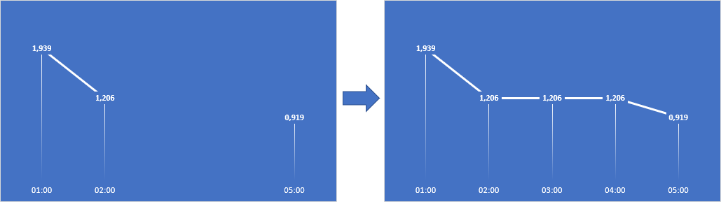
Here, the spontaneous value applies to all underlying raster points:

The value of 02:00-05:00 is therefore rolled out for hours 2, 3 and 4 as follows:

Roll out with aggregation rule Sum

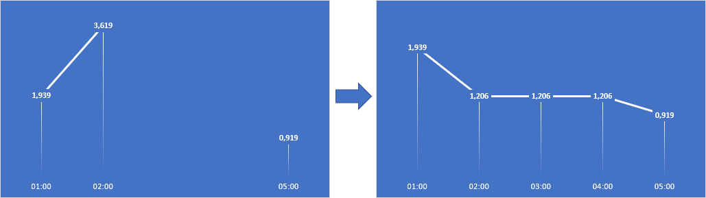
Here, the spontaneous value applies proportionally to all underlying raster points:

The value of 02:00-05:00 is thus rolled out proportionally for hours 2, 3 and 4 as follows:

Begin Vs. End Time Series

Begin time series represent time series where a value is available at the beginning of the respective measuring period. This is the case, for example, with power values (watts). Begin time series can also be used to represent momentary values (such as temperature, wind speed, length, etc.) that are valid at the time of measurement. 

End time series represent time series where a value is available at the end of the respective measuring period. This is for example the case with energy values (watt hour).

Depending on the time series type, the respective value is referenced in the database with the start time stamp (from value concept) or with the end time stamp (to value concept). Since currently all values are visualized in data queries as from timestamp-value pairs or as from-to timestamp-value pairs, this distinction into begin and end time series types can be seen as a pure classification. 

We recommend the following videos under Video Tutorials:

• Types of Time Series

• Formula Time Series

• Historization of Time Series Data